2.4 Applying the basic patterns

Now we will show a popular example, introduce a library called NumPy, and suggest a problem for you to solve by filling in some code.

Trapezoidal Rule Integration with Message Passing

This problem is also shown in Chapter 1, section 1.3, with a shared memory solution in OpenMP. The algorithm is a straightforward mathematical technique for finding the area under a curve by splitting the area into many small trapezoid slices whose area we can estimate, then add those areas together. This type of numerical integration is described on Wikipedia using the following diagram for an arbitrary function:

Consult the above Wikipedia entry for details on the mathematics for the composite trapezoidal rule, which is written into the function called trapSum() in the code below.

In our case, we will begin by considering the sine(x) function, which looks like this when x varies from 0 to \(5*\pi\):

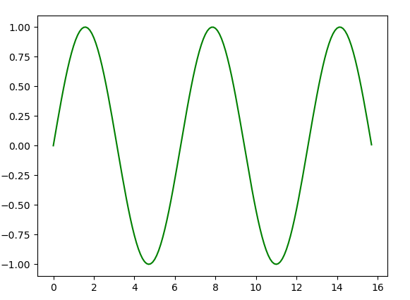
We will use this function to make it simpler for us to determine the correctness of our parallel implementation in MPI. To make it even simpler, let’s first concentrate on the range of the first part of the above function, from 0 to \(\pi\), which looks like this:

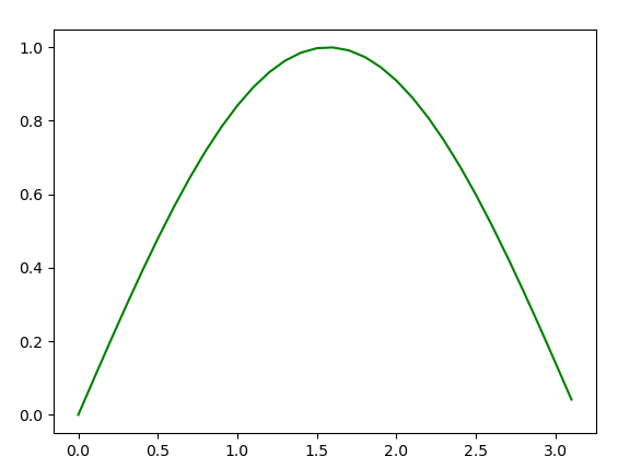
We will rely on a mathematical theory which tells us that the integral where x ranges from 0 to \(\pi\) of sine(x) is 2.0. A sequential solution would split the curve of this function into many small trapezoids, iterating from a = 0.0 to b = \(\pi\), summing the value of each trapezoid as we go.

The code below illustrates how the trapezoidal integration example could be implemented with point-to-point communication. In this case, each process, including the conductor, splits up the computation among themselves using the parallel for loop pattern.

To visualize this, suppose we were using a small number of trapezoids (24) and 4 processes. We can decompose the work so that each process works on computing 6 of the trapezoids, like this, where each color represents a process:

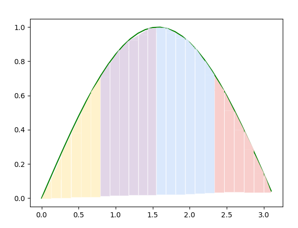
All of the processes add up the areas of their portion of the function, \(sine(x)\). Note that, as in the picture above, each process will determine its local range of values of x, my_a, and my_b. The workers send their ‘local’ sum to the conductor. Then the conductor waits to receive data from each of the other processes and combines the data received to calculate the final answer.

from mpi4py import MPI import math #constants n = 1048576 #number of trapezoids = 2**20 def f(x): return math.sin(x) def trapSum(my_a, my_b, my_n, h): my_a*=h my_b*=h total = (f(my_a) + f(my_b))/2.0 #initial value for i in range(1, my_n): #for each trapezoid total += f(my_a+i*h) return total*h def main(): comm = MPI.COMM_WORLD id = comm.Get_rank() numProcesses = comm.Get_size() #desired range a, b = 0, math.pi # all processes: compute local variables ############################################# local_n = int(n/numProcesses) #num trapezoids per process isTail = n % numProcesses start = id*local_n #starting trapeziod end = (id+1)*local_n #ending trapezoid #in case processors cannot divide things evenly if id == numProcesses-1 and isTail > 0: end = n h = (b-a)/n #width of trapezoid (scaling factor) # all processes: calculate local sum ################################################# my_sum = trapSum(start, end, local_n, h) # if a worker process, send ######################################### if id != 0: comm.send(my_sum, dest=0) #send conductor the sum # conductor process else: results = [0.0]*numProcesses #generate conductor list to hold results results[0] = my_sum #places conductor's local sum in first element for i in range(1,numProcesses): other_sum = comm.recv(source=i) #get local sums from other processes results[i] = other_sum #place in result array print("Done receiving all messages") print("Final sum is {0}".format(sum(results))) ########## Run the main function main()

The trapSum() function computes and sums up a set of n trapezoids with a particular range. The first part of the main() function follows the SPMD pattern. Each process computes its local range of trapezoids and calls the trapSum() function to compute its local sum.

The latter part of the main() function follows the conductor-worker pattern. Each worker process sends its local sum to the conductor process. The conductor process generates a global array (called results), receives the local sum from each worker process, and stores the local sums in the results array. A final call to the sum() function adds all the local sums together to produce the final result.

Note

Notice lines 30, 36, and 37 in the code above. We use this technique to ensure that we can use any number of trapezoids and any number of processes, even if the trapezoids do not divide evenly among the processes. Compare this to the previous section, where we insisted that they divide evenly. Handling the case where we may have extras from non-even division of loops is a preferred parallel programming practice.

Try improving the result

This code is computing the integral from 0 to \(\pi\) of \(sine(x)\), which from mathematical theory should be 2.0. Notice the difference in the result if you increase the number of trapezoids, n on line 5 by multiplying it by 8, changing it to n = 1048576*8. Is this a better approximation of the result?

In later sections, we will see how to improve this example with other communication constructs. For now, ensure that you are comfortable with the workings of this program.

A Brief Aside: the numpy library

The mpi4py library of functions has several collective communication functions that are designed to work with arrays created using the Python library for numerical analysis computations called NumPy. Unlike Python lists, NumPy arrays hold only one type of data, and generally are faster and take up less space than Python lists that contain data of only one type.

NumPy arrays are specifically designed for fast mathematical computations and can be reshaped to form matrices and other multi-dimensional data structures. A detailed discussion of NumPy is beyond the scope of this book; for more about its features and available methods, we recommend consulting the documentation and available tutorials.

Since we do need some basic idea of how NumPy arrays work, however, let’s examine the following Python program that creates arrays in two different ways and displays them. We start with the import of numpy as np. Note how we make a point that some numpy functions expect their inputs to be certain types– for example, np.empty() takes an integer for the length of a new array to create.

import numpy as np # array size to use below length = 20 def main(): #initialize using numpy function, length must be an integer type npArray = np.empty(length) # put increasing float values into array for i in range(len(npArray)): next = float(i) npArray[i] = next # array syntax print('Array contains values of type:') print(npArray.dtype) print(npArray) sumVals = 0.0 for val in npArray: sumVals = sumVals + val print("Sum from loop = {}, sum from python function = {}"\ .format(sumVals, sum(npArray) )) # an alternative way to create simple increasing values data = np.linspace(0, #start length - 1 , #stop length, #total elements dtype='u4') # 4-byte unsigned integer data type print("alternative form of creating array produces:") print(data) print("whose sum is: {}".format(np.sum(data))) main()

After running this example, compare the code to the output. Observe that numpy library arrays have these characteristics:

• Arrays are created to have a given length.

• Arrays always contain values of a certain numerical type.

• We use syntax like this to access the i_th value of an array: npArray[i]

Exercise - Populate an Array

As an exercise, let’s use point-to-point communication to populate an array in parallel. Suppose we want to generate an array of N values from 1 to N. For typical real problems, N is large and may have a random pattern of values. But to visualize what you need to do for this simpler version, if N was 9 and we had 3 processes, each process could create part of the desired final array in local arrays like this:

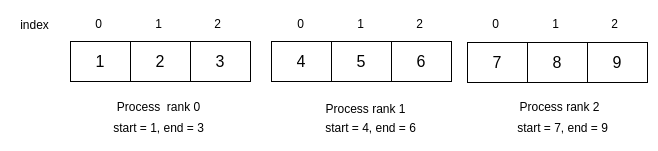
Once each worker process has created its local portion of the overall array, it can send that to the conductor, who will place it in the proper location in a global array of length 9 that it has created.

Note

The important points about coding a correct solution for p processes are

1. The local array in each process contains N/p values, thus its length is an integer equal to N/p.

2. We use the process rank and the number of elements in each local array to determine its start value and end data values, which will be integers. Take the time now to determine how to compute a start and end data value.

3. In case N is not divisible by p, the last process can create N%p extra values. This technique will also be used in later sections of this chapter.

Use what you have seen in the previous examples to determine how to split up the loop in the populateArray function below. The algorithm is as follows

1. Each process computes its local range of values by calling a populateArray function that generates an array of just those values.

1. Each process populates an array of N/p values, where p is the number of processes. In other words, the number of elements (nElems) in each local array is N/p.

2. Each process determines its start and end values and length of their array:

3. Process 0 generates values 1 through nElems,

4. Process 1 generates values nElems+1 through 2*nElems

5. etc. for each process chosen

2. Each worker process sends its array to the conductor process.

3. The conductor process generates a global array of the desired length, receives the local array from workers, and then populates the global array with the elements of the local arrays received.

4. The final global array on the conductor has N values, simply holding all values from 1 to N.

The following program is a partially filled in solution, with the parts to complete shown in comments with TODO beside them. If you are stumped, a solution is hidden below.

from mpi4py import MPI import numpy as np #array size N = 1600 # using the global N for the array size, # determine the number of elements the process # running this function will make. # The fill the local array of N/p elements. # Step 1 in algorithm description def populateArray(rank, nprocs): #declare local variables: # number of elements to generate must be an int so length stays an int nElems = int(N/nprocs) start = # TODO: starting element end = # TODO: end element length = # TODO: length of array to generate # TODO: if I am the last process, update end to hold N%p extra values #generate empty array local_array = np.empty(length) #fill with desired values (start+1..end+1) for i in range(length): local_array[i] = # TODO: value at index i based on start return local_array def main(): comm = MPI.COMM_WORLD myId = comm.Get_rank() numProcesses = comm.Get_size() #SPMD pattern - all processes create data local = populateArray(myId, numProcesses) #generate a local array #conductor-worker pattern/send-receive # first the worker should send (step 2) if (myId != 0): # TODO: send local array to conductor else: # conductor step 3 of algorithm # conductor makes global array, and fills with zeroes global_array = np.empty(N) #copy conductor's local array to global for i in range(len(local)): global_array[i] = local[i] pos = len(local) # index in global for local array from worker 1 # TODO: receive local arrays from each worker into a temp array, # and merge into global_array, updating pos as # start of where to copy into global for i in range(1, numProcesses): #solution check: the two sums should be equal total = int(sum(global_array)) print(total) print((N*(N+1)/2)) ########## Run the main function main()

Fill in the rest of the program, test your program using 1, 2, 3, and 4 processes. For initial debugging, you might want to temporarily change N to a small number like 9 and print out the local arrays in each process and the global array on the conductor.

Remember, in order for a parallel program to be correct, it should return the same value with every run, regardless of the number of processes chosen. Click the button below to see our solution.

Warning

If you have errors in your code, you may simply get output that looks like this:

===== NO STANDARD OUTPUT =====
===== NO STANDARD ERROR =====

You will need to try a fix. It is best to work on each TODO task, perhaps adding a debug print, try running to be sure you haven’t introduced an error before you go on.

Solution

The following program demonstrates how to implement the populateArray program. Make sure you try to solve the exercise yourself before looking at the solution!

from mpi4py import MPI import numpy as np #array size N = 1600 def populateArray(rank, nprocs): nElems = int(N/nprocs) #number of elements to generate isTail = N % nprocs start = rank*nElems end = (rank+1)*nElems if rank == (nprocs-1) and isTail > 0: end = N length = end-start local_array = np.empty(length) for i in range(length): local_array[i] = 1+start+i return local_array def main(): comm = MPI.COMM_WORLD myId = comm.Get_rank() numProcesses = comm.Get_size() #SPMD pattern local = populateArray(myId, numProcesses) #generate an empty array of size N #conductor-worker pattern/send-receive if (myId != 0): comm.send(local, dest=0) else: #initialize global array, and fill with conductor's elements global_array = np.empty(N) for i in range(len(local)): global_array[i] = local[i] pos = len(local) #merge into one array for i in range(1, numProcesses): loc = comm.recv(source=i) for j in range(len(loc)): global_array[pos+j] = loc[j] pos += len(loc) #print out final array total = int(sum(global_array)) print(total) ########## Run the main function main()

You have attempted of activities on this page