
6.2 Trapezoidal Rule Integration with MPI
Our next example is also a classic for demonstrating parallel computing, and we introduced it already in our companion PDC for Beginners book using OpenMP for a shared memory system.
The algorithm is a straightforward mathematical technique for finding the area under a curve by splitting the area into many small trapezoid slices whose area we can estimate, then add those areas together. This type of numerical integration is described on Wikipedia using the following diagram for an arbitrary function:

Consult the above Wikipedia entry for details on the mathematics for the composite trapezoidal rule, which is written into the function called Trap() in the code below.
In our case, we will begin by considering the sine(x) function, which looks like this when x varies from 0 to \(5*\pi\):
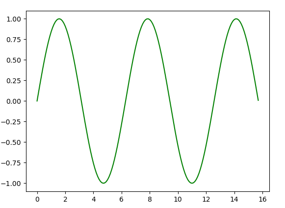
We will use this function to make it simpler for us to determine the correctness of our parallel implementation in MPI. To make it even simpler, let’s first concentrate on the range of the first part of the above function, from 0 to \(\pi\), which looks like this:
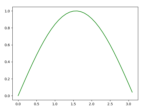
We will rely on a mathematical theory which tells us that the integral where x ranges from 0 to \(\pi\) of sine(x) is 2.0. A sequential solution would split the curve of this function into many small trapezoids, iterating from a = 0.0 to b = \(\pi\), summing the value of each trapezoid as we go. This is provided in a function called Trap(), which looks like this:
double Trap(double left_endpt, double right_endpt, int trap_count, double base_len) {
    double estimate, x;
    int i;

    estimate = (f(left_endpt) + f(right_endpt))/2.0;
    for (i = 1; i <= trap_count-1; i++) {
        x = left_endpt + i*base_len;
        estimate += f(x);
    }
    estimate = estimate*base_len;
    return estimate;
}
In this case, base_len is the width of each trapezoid, trap_count is the number of trapezoids, and left_endpt and right_endpt are the range we will be integrating over.
Parallelize with common patterns
Perhaps unsurprisingly, the patterns used in this solution are the same as the previous Monte Carlo example, because we again have a familiar for loop in this above function that we can decompose into chunks.
The important patterns in this code are:
SPMD, since we have one program that multiple processes all run.
Data decomposition, since each process will compute an equal share of the total number of trapezoids requested.
Parallel for loop split with equal chunks computed by each process.
Reduction communication pattern to combine the results from each process.
There is also a broadcast from process 0. See if you can find that and what it was used for.
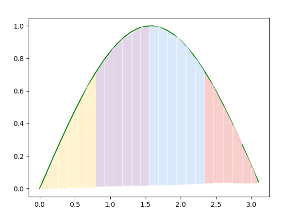
To illustrate the use of these patterns, suppose we were using a small number of trapezoids (24) and 4 processes. We can use decomposition of the loop in the Trap() function above so that each process works on computing 6 of the trapezoids, like this, where each color represents a process:
In the following code example, focus on the use of ‘local’ in certain variables below. These indicate values that will be different for each process and represent the range of values that each process can compute. Each process keeps its own sum for the area of the trapezoids, and then the reduction takes place when all processes are completed.