6.1 A simple Monte Carlo simulation¶

This first MPI example is a classic- you will find many, many examples of it on the web, and it is used to describe Monte Carlo methods on Wikipedia, where the following image is found (click for its attribution):

The method is straight forward:

Consider one quarter of a unit circle (a quadrant) inscribed inside a square of width 1.0.
Randomly choose x, y between 0.0 and 1.0 of a point and determine if the point lies within or outside the quadrant.
Keep choosing points.
When done, compute the ratio of the points inside the circle to the total number of points. This is an estimate of the ratio of the area of the circle quadrant to the square, which we know to be \(\pi/4\).
We can estimate the value of \(\pi\) by multiplying by 4.

From steps 2 and 3 above, you can infer that there is a loop where a given number of random points are generated and counted as in or out. This type of loop makes this algorithm a candidate for decomposition using a parallel for loop pattern. The following code demonstrates this. In addition, we show how we can use the parallel random number generator library introduced in Chapter 3 in an MPI program- it is very similar to how we used it for the basic OpenMP examples that we showed there.

Primary patterns used¶

The important patterns to envision in this code are:

SPMD, since we have one program that multiple processes all run.
Data decomposition, since each process will compute an equal share of the total number of points requested.
Parallel for loop split with equal chunks computed by each process (inside the function called Toss()).
Reduction communication pattern to combine the results from each process.
There is also a broadcast from process 0. See if you can find that and what it was used for.

We start with this relatively straightforward example to illustrate that most MPI applications contain several patterns like this.

/*
* Hannah Sonsalla, Macalester College, 2017
* Libby Shoop updated to use trng
*
*  calcPiMPI.C
*
*   ...program uses MPI to calculate the value of Pi
*
* Usage:  mpirun -np N ./calcPiMPI <number of tosses>
*
* Note that this uses the block splitting technique for
* generating random numbers. This requires that the number
* of tosses be equally divisible by the number of processes.
*
*/

#include <mpi.h>
#include <math.h>
#include <stdio.h>
#include <stdlib.h>
#include <time.h>
#include <trng/yarn2.hpp>
#include <trng/uniform01_dist.hpp>

void Get_input(int argc, char* argv[], int myRank, long* totalNumTosses_p);
long Toss (long numProcessTosses, int myRank);

int main(int argc, char** argv) {
    int myRank, numProcs;
    long totalNumTosses, numProcessTosses, processNumberInCircle, totalNumberInCircle;
    double start, finish, loc_elapsed, elapsed, piEstimate;
    double PI25DT = 3.141592653589793238462643;         /* 25-digit-PI*/

MPI_Init(&argc, &argv);
    MPI_Comm_size(MPI_COMM_WORLD, &numProcs);
    MPI_Comm_rank(MPI_COMM_WORLD, &myRank);

// Read total number of tosses from command line
    Get_input(argc, argv, myRank, &totalNumTosses);

// check for equal chunks per processor, since
    // block splitting requires this
    // only one process needs to print the error
    //
    if ((totalNumTosses % numProcs) == 0) {
        // how many tosses each process will complete
        numProcessTosses = totalNumTosses/numProcs;
    } else {
        if (myRank == 0) {
            printf("Number of tosses must be divisible by number of processors. Exiting.\n");
        }
        MPI_Finalize();
        exit(-1);
    }

MPI_Barrier(MPI_COMM_WORLD);  // start timing
    start = MPI_Wtime();

processNumberInCircle = Toss(numProcessTosses, myRank);

MPI_Reduce(&processNumberInCircle, &totalNumberInCircle, 1, MPI_LONG, MPI_SUM, 0, MPI_COMM_WORLD);

// Get the highest time as the final end time
    finish = MPI_Wtime();
    loc_elapsed = finish-start;
    MPI_Reduce(&loc_elapsed, &elapsed, 1, MPI_DOUBLE, MPI_MAX, 0, MPI_COMM_WORLD);

if (myRank == 0) {
        piEstimate = (4*totalNumberInCircle)/((double) totalNumTosses);
        printf("Elapsed time = %f seconds \n", elapsed);
        printf("Pi is approximately %.16f, Error is %.16f\n", piEstimate, fabs(piEstimate - PI25DT));
    }
    MPI_Finalize();
    return 0;
}

/* Function implements Monte Carlo version of tossing darts at a board */
// Each process runs this.
// Each time through a loop the process creates a set of random x, y values
// between 0.0 and 1.0 from its block determined by the trng jump function.
long Toss(long processTosses, int myRank){
    long numberInCircle = 0;
        double x,y;
        unsigned long int seed = (unsigned long int) time(NULL);
    trng::yarn2 r;

r.seed(seed);

trng::uniform01_dist<> u; // random number distribution
    r.jump(2*(myRank*processTosses));   // jump ahead to set of
                                        // random values for my process:
                                        // this is block splitting
    // throw random points into square and distribute workload over all processes
    for (long i=myRank*processTosses; i<(myRank+1)*processTosses; ++i) {
        x=u(r);
        y=u(r); // choose random x, y coordinates
        if (x*x+y*y<=1.0) {      // is point in unit circle ?
            ++numberInCircle; // increase counter
        }
    }
    return numberInCircle;
}

/* Function gets input from command line for totalNumTosses */
void Get_input(int argc, char* argv[], int myRank, long* totalNumTosses_p){
    if (myRank == 0) {
        if (argc!= 2){
            fprintf(stderr, "usage: mpirun -np <N> %s <number of tosses> \n", argv[0]);
            fflush(stderr);
            *totalNumTosses_p = 0;
        } else {
            *totalNumTosses_p = atoi(argv[1]);
        }
    }
    // Broadcasts value of totalNumTosses to each process
    MPI_Bcast(totalNumTosses_p, 1, MPI_LONG, 0, MPI_COMM_WORLD);

// 0 totalNumTosses ends the program
    if (*totalNumTosses_p == 0) {
        MPI_Finalize();
        exit(-1);
    }
}

Here are some things to note about this code:

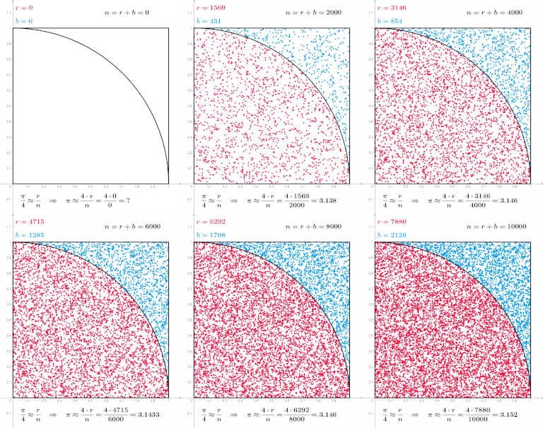
The function called Toss is named that because choosing the numbers is like tossing a dart at the square. Though our use of random numbers makes the tosses far more uniform than a human on a real board.
The command line argument is the number of random ‘tosses’ to generate.
We illustrate the block-splitting approach for delving out random numbers to the processes. The default value of 200000 tosses is divisible by 2, 4, and 8 threads so that this will work. We have a check to make sure that the number of tosses is divisible by the number of processes chosen.
We use the -Ofast compiler flag because in our experience the trng random number generator functions seem to perform better using this.

Exercises

Try increasing the number of tosses from 200000 to 2000000, then 20000000, then 200000000, and finally 2000000000 by adding a 0 each time and re-running with 4 or 8 processes. Does the estimated value of pi get more accurate as you increase the number of tosses? NOTE: random number generators have a limit of how many numbers they can generate. If you try too many, it will fail mysteriously.
For a challenge: Try changing to the leapfrog method for generating the random values, using the method called ‘split’. Revisit how this was done in Chapter 3.
For a challenge: Try using a different random number generation class from the trng library other than yarn2.

You have attempted of activities on this page