
5.3 Exploring the effect of block and grid size settings
Each of the following sections describes with illustrations and small code snippets how we can set up different block sizes (numbers of threads per block) and different grid sizes (blocks per grid) for this code example.
Note
We illustrate these examples because you may see code examples like this when you search for examples to help you. Particular approaches may be more effective, but ultimately you want to try some tests like this for your particular GPU card.
Recall from Chapter 4 that the CUDA programming model is designed for blocks of threads to be used on Streaming Multiprocessers (SMs) as shown in Figure 4-3 and repeated here:
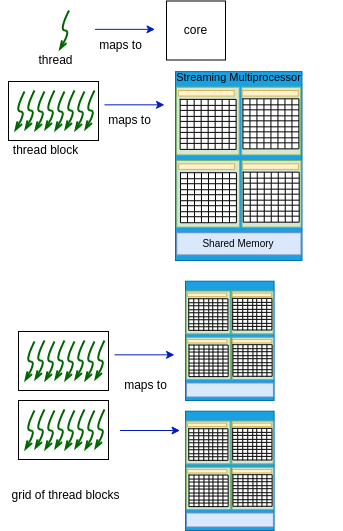
Figure 4-3. CUDA Programming model
In prior examples in the previous chapter, we used one way of mapping the threads to compute each element of the array. We will explore different mappings of thread blocks in a 1D grid to a 1D array that represents vectors to be added together.
Case 3: Using a single block of threads
We’ll start by envisioning the simplest case from earlier examples, a single block of 8 threads as shown in Figure 5-1.
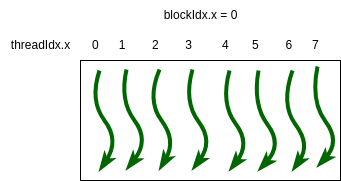
Figure 5-1. A simple 1D grid with one block of 8 threads.
Suppose that we are adding an array of 16 elements to another array of 16 elements using the algorithm for vector addition. There are different ways of setting up a grid of block(s) to complete this task. The first is shown in Figure 5-2, where a single block of 8 threads can be mapped over time to complete 8 computations simultaneously. An example kernel function to do this is shown just below it.
In this case, the block of green threads first works on the first 8 elements of the array. Then in a next larger time step, the block of threads shown in a magenta color would complete the work.
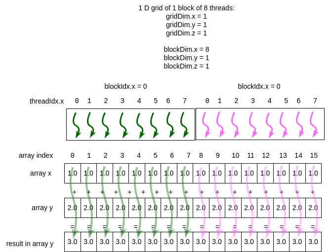
Figure 5-2 Using one block means less parallelism
The kernel function for this is as follows:
// Parallel version that uses threads in the block.
//
//  If block size is 8, e.g.
//    thread 0 works on index 0, 8, 16, 24, etc. of each array
//    thread 1 works on index 1, 9, 17, 25, etc.
//    thread 2 works on index 2, 10, 18, 26, etc.
//
// This is mapping a 1D block of threads onto these 1D arrays.
__global__
void add_parallel_1block(int n, float *x, float *y)
{
  int index = threadIdx.x;    // which thread am I in the block?
  int stride = blockDim.x;    // threads per block
  for (int i = index; i < n; i += stride)
      y[i] = x[i] + y[i];
}
Pay particular attention to the for loop and how index and stride are set up. Compare the code to the diagram, where the single block is repeated over the top of the array elements it will work on. For 32 elements, imagine 4 larger time steps in this loop, with 8 threads in the block ‘sliding along’ to work on the next 8 elements. It is used in main like this, with 1 block specified in the kernel function call:
add_parallel_1block<<<1, blockSize>>>(N, x, y); // the kernel call
Note
It’s important to understand that the CUDA runtime system takes care of assigning the block of threads to ‘slide along’ your array elements. As a programmer, you are setting up the loop for this and specifying one block. This limits the overall parallelism, mainly because one block runs on one SM on the device, as shown in Figure 4-3 above.
Case 4: Using a small fixed number of multiple blocks of threads
Using multiple blocks of threads in a 1D grid is the most effective way to use an NVIDIA GPU card, since each block will map to a different streaming multiprocessor. Recall this figure from section 4-2:
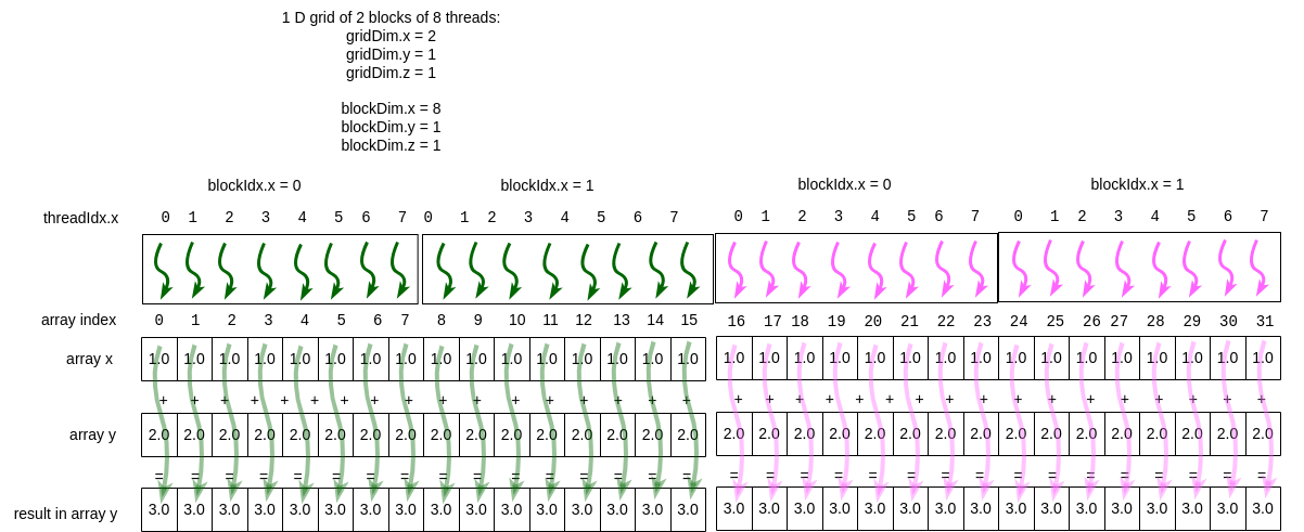
Figure 5-3 CUDA programming model for using multiple blocks
There are different ways of using multiple blocks of threads in our kernel function code. One way is to set a fixed number of blocks in the grid. Let’s illustrate this with an example. Suppose that we use 2 blocks of 8 threads each when we call a kernel function. Further suppose that we have 32 elements in our arrays. This situation is shown in Figure 5-3 Note how with 2 blocks of 8 threads we can perform 16 computations in parallel, then perform 16 more.
Note that if we increase our array size, for example by doubling it to 64, yet keep the same grid size and block size, the picture above would need four colors to depict the computations that can happen in parallel (in theory- see note below).
The kernel function for this case is as follows:
// In this version, thread number is its block number
// in the grid (blockIdx.x) times
// the threads per block plus which thread it is in that block.
//
// Then the 'stride' to the next element in the array goes forward
// by multiplying threads per block (blockDim.x) times
// the number of blocks in the grid (gridDim.x).

__global__
void add_parallel_nblocks(int n, float *x, float *y)
{
  int index = blockIdx.x * blockDim.x + threadIdx.x;
  int stride = blockDim.x * gridDim.x;
  for (int i = index; i < n; i += stride)
    y[i] = x[i] + y[i];
}
It is used in main like this:
  // Number of thread blocks in grid could be fixed
  // and smaller than maximum needed.
  int gridSize = 16;

  printf("\n----------- number of %d-thread blocks: %d\n", blockSize, gridSize);

  t_start = clock();
  // the kernel call assuming a fixed grid size and using a stride
  add_parallel_nblocks<<<gridSize, blockSize>>>(N, x, y);
Note that the gridSize and blockSize variables above are simply integers and not of type dim3. This shortcut is often used by CUDA programmers when using 1D arrays.
Note
One could argue that the above depiction is not strictly true. The CUDA block scheduler on many devices has gotten really good at making the ‘stride’ version of the code with a fixed grid size run nearly as fast as the following example (case 5 below). You will likely observe this when you run it. It may not be true for other applications, however, so you always need to check and test like we are doing here.
The reason for this is that every core in an SM can actually run multiple threads simultaneously. So the hardware scheduler can assign blocks to run simultaneously on an SM, apparently as efficiently as if the blocks were spread across all SMs, at least for this example and for higher-end GPU cards. So our picture in Figure 4-3 is too simple for modern NVIDIA GPU devices when it comes to scheduling the running threads. The running of the threads is more like Figure 5-4.
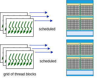
Figure 5-4. CUDA schedules blocks to run simultaneously
A technical post from NVIDIA states this:
One SM can run several concurrent CUDA blocks depending on the resources needed by CUDA blocks.
We provide this example because you will likely see code examples written like this as you scour the web for CUDA examples. And you may find that some applications perform just a bit better using it. The next method, however, follows what you have seen already: calculate the number of blocks in the grid based on a block size and the number of elements in the array. In theory, this enables you to scale your problem and to use as many streaming multiprocessors on your device as possible.
Case 5: Variable grid size method
As the arrays become larger or smaller for a given problem you are working on, or you choose a different number of threads per block (a useful experiment to try for any card you are using), an alternate method is to use the array size and the block size to compute the needed 1D grid size.
Though the execution time of this and the previous method may be similar, this method is shown in a lot of examples and is a useful way to think about CUDA programs: create all the threads you need and map every thread to a particular index in the array.
For example, in the case in Figure 5-3, we looked at doubling the size of the array, but keeping the same number of blocks of threads. Now let’s suppose that we compute a new grid size (blocks per 1D grid) based on the array size and number of threads per block. In this case, we would have the situation given in Figure 5-5. From this, note that we have only one color for the threads because all of the calculations can be done in parallel.
So as the problem size (length of the array in this case) grows, we should be able to take full advantage of the architecture.
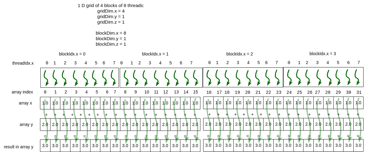
Figure 5-5 Number of blocks based on array size and block size
Here is the corresponding kernel function for this (similar to the previous chapter):
// Kernel function based on 1D grid of 1D blocks of threads
// In this version, thread number is:
//  its block number in the grid (blockIdx.x) times
// the threads per block plus which thread it is in that block.
//
// This thread id is then the index into the 1D array of floats.
// This represents the simplest type of mapping:
// Each thread takes care of one element of the result
//
// For this to work, the number of blocks specified
// times the specified threads per block must
// be the same or greater than the size of the array.
__global__
void vecAdd(float *x, float *y, int n)
{
    // Get our global thread ID
    int id = (blockIdx.x * blockDim.x) + threadIdx.x;

    // Make sure we do not go out of bounds
    if (id < n)
        y[id] = x[id] + y[id];
}
Note that there is no stride variable used in the kernel function, which is used in main like this:
  // set grid size based on array size and block size
  gridSize = ((int)ceil((float)N/blockSize));

  printf("\n----------- number of %d-thread blocks: %d\n", blockSize, gridSize);

  t_start = clock();
  // the kernel call
  vecAdd<<<gridSize, blockSize>>>(x, y, N);
Note
Using this method, as array sizes get very large, the grid size needed will exceed the number of SMs on your device. However, as we mentioned before, the system will take care of re-assigning cores on an SM to a new portion of the computation for you.
Let’s test your recollection of how kernel functions are called in main without using variables of type dim3.
- It is valid and will run using a 1D grid of 128 blocks of 1000 threads each.
- Look at the case 4 and 5 kernel function calls in main.
- It is valid and will run using a 1D grid of 1000 blocks of 128 threads each.
- Yes! The grid size as an integer can be used and is the first argument.
- It is invalid.
- Note how two cases above do not use dim3 arguments.
5.3-1: Which is true about the following kernel function call?
vecAdd<<<1000, 128>>>(x, y, N);
Let’s now see these cases in action in the next section.