2.9 Real World Example - Forest Fire Simulation

Ported to Python by Libby Shoop (Macalester College), from the original [Shodor foundation C code example](http://www.shodor.org/refdesk/Resources/Tutorials/BasicMPI/).

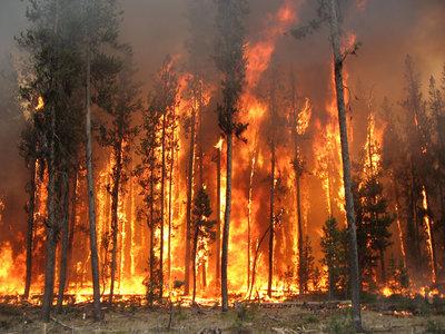
The goal is to simulate a forest fire using an N x N grid of trees. If a tree starts to smolder, each tree around it has some chance of catching fire. The model follows the following set of rules (from Shodor):

• Burning trees burn down.

• Smoldering trees catch fire.

• Unburnt trees next to (N, S, E, W) a burning tree catch fire with some random probability less than or equal to a given probability threshold.

• Repeat until fire burns out.

The main input parameters for the model are:

• The size, N of one row of trees in the N x N grid representing part of the forest.

• The upper limit of the chance of the fire spreading from a burning tree to a nearby unburnt tree.

The simulation of one tree burning starts with the tree in the center of the grid smoldering, and all other trees alive.

The main outputs for the single fire model are:

• The percentage of additional trees burned beyond the first tree.

• The number of iterations before the fire burns out.

The fire functions

There are several functions that a single fire simulations uses, and they are in the following code block for reference.

import numpy as np UNBURNT = 1 BURNT = 0 SMOLDERING = 2 BURNING = 3 def initialize_forest(size): """ Create the forest of unburnt trees as a 2D array Parameters: size (int): number of trees in each row and column Returns: size x size numpy array """ forest = np.empty( (size, size), dtype='u4') forest.fill(UNBURNT) return forest def light_tree(row_size, forest, x, y): """ Tree at position x, y in forest set to smoldering Parameters: row_size (int): number of trees in each row and column forest (array): array representing the 2D forest x (int), y (int): x,y location of tree to set smoldering post[forest]: If x, y is properly within the array, the tree at x, y is set. Otherwise, one tree in the center of the forest is set. """ # note that indexes into numpy arrays must be integers if x >= row_size or y >= row_size : print("Warning: starting position out of bounds; using center") i = int(row_size/2) j = int(row_size/2) else: i = int(x) j = int(y) forest[i,j] = SMOLDERING def fire_spreads(prob_spread): """ Generates a random number between 0 an 1 and checks if < prob_spread Parameters: prob_spread (float): probability threshold for determining whether burning tree will spread to neighboring tree Returns: True if new random value is < prob_spread, False otherwise """ prob = np.random.random_sample() if prob < prob_spread: return True else: return False def forest_burns(forest, row_size, prob_spread): """One round of burning the forest Sets every burning tree to burnt, and every smoldering tree to burning. Then sets fire to unburt trees next to burning trees randomly, based on the probability of spreading. Parameters: forest (array): array representing the 2D forest row_size (int): number of trees in each row and column prob_spread (float): probability threshold for determining whether burning tree will spread to neighboring tree """ # burning trees burn down, smoldering trees ignite for index, value in np.ndenumerate(forest): # print(forest[index], value) #debug if forest[index] == BURNING: forest[index] = BURNT if forest[index] == SMOLDERING: # print(index, " SMOLDERING") #debug # print(index[0], index[1]) forest[index] = BURNING for index, value in np.ndenumerate(forest): i, j = index[0], index[1] # row, col, location in grid # unburnt trees surrounding burning trees catch fire if # random probability is above threshold of probability of spreading if forest[index] == BURNING: if i != 0 : #check tree to north if not on top row if forest[(i-1, j)] == UNBURNT and fire_spreads(prob_spread): forest[(i-1, j)] = SMOLDERING if i != row_size-1 : #check tree to south if not on last row if forest[(i+1, j)] == UNBURNT and fire_spreads(prob_spread): forest[(i+1, j)] = SMOLDERING if j != 0 : #check tree to west if not on left side if forest[(i, j-1)] == UNBURNT and fire_spreads(prob_spread): forest[(i, j-1)] = SMOLDERING if j != row_size-1 : #check tree to east if not on right side if forest[(i, j+1)] == UNBURNT and fire_spreads(prob_spread): forest[(i, j+1)] = SMOLDERING def forest_is_burning(forest): """ Checks for any remaining smoldering or burning trees Parameters: forest (array): array representing the 2D forest Returns: True if at least one tree is still in burning or smoldering state. False if all trees are burnt. """ for row in forest: for tree in row: if tree == SMOLDERING or tree == BURNING: return True return False def get_percent_burned(forest, row_size): """ Determine how many trees burned during fire Parameters: forest (array): array representing the 2D forest row_size (int): number of trees in each row and column Returns: percent : float Percentage of total number of trees that were burned, as a float between 0 and 1. """ sum = 0 for row in forest: for tree in row: if tree == BURNT: sum +=1 return float(sum)/float(row_size*row_size) def print_forest(forest): """ Ascii display of forest Prints values for state of each tree in the forest. Parameters: forest (array): array representing the 2D forest """ for row in forest: rowStr = '' for tree in row: if tree == BURNT: rowStr = rowStr + '.' elif tree == UNBURNT: rowStr = rowStr + 'Y' elif tree == SMOLDERING: rowStr = rowStr + 'S' else: rowStr = rowStr + 'B' print(rowStr) print('\n')

A single fire burning

# # Run one simulation of a fire burning at one probability threshold. # # Ported to python from the original Shodor foundation example: # http://www.shodor.org/refdesk/Resources/Tutorials/BasicMPI/ # # Libby Shoop Macalester College # import argparse # for command-line arguments def parseArguments(): """Handle command line arguments Run with -h to get details of each argument. Returns: A list containing each argument provided """ # process command line arguments # see https://docs.python.org/3.3/howto/argparse.html#id1 parser = argparse.ArgumentParser() parser.add_argument("numTreesPerRow", help="number of trees in row of square grid") parser.add_argument("probabilityOfSpread", help="probability threshold of fire spreading from one burning tree to a non-burning tree next to it (percent between 0 and 1)") # could add: optional arguments for i, j position of starting tree args = parser.parse_args() row_size = int(args.numTreesPerRow) prob_spread = float(args.probabilityOfSpread) return row_size, prob_spread ############################# main() ########################## def main(): row_size, prob_spread = parseArguments() forest = initialize_forest(row_size) percent_burned = 0.0 # for now start burning at midlle tree middle_tree_index = int(row_size/2) light_tree(row_size, forest, middle_tree_index, middle_tree_index) iter = 0 # how many iterations before the fire burns out while forest_is_burning(forest): # print("burning") # debug forest_burns(forest, row_size, prob_spread) iter += 1 percent_burned = get_percent_burned(forest, row_size) print("Iterations until fire burns out: {}".format(iter)) print("Percent burned: {0:4.3f}".format(percent_burned)) print_forest(forest) ########## Run the main function main()

The first command line argument in the code block above represents the length of one row, N, of an NxN forest.

The second argument is the probability threshold of spreading. In the forest_burns() function, if a tree is burning and its neighbor is not, a random number between 0 and 1.0 is generated for whether the neighbor will catch fire. If the number is less than the probability threshold, the tree is set to smolder.

The output of running the above single fire shows an approximation of how long it takes for the fire to burn out by counting the number of times the function forest_burns() executes. This is given as the iterations until the fire burns out.

The next part of the output shows the percentage of trees in the forest burned on this particular trial.

Lastly, a textual output of what the final forest looks like is shown, where a ‘Y’ is a live tree and a ‘.’ is a dead tree.

Warning

In this case, this program should run on only one process, so please do not change the -np mpirun flag.

Exercises

One single instance of this one-fire model can produce a different result each time it is run because of the randomness of the probability of unburnt trees catching fire.

1. Try running this several times at the same 0.5 threshold. Notice how the iterations and the percent burned changes.

2. Try varying the threshold from 0.2 to 1.0 by 0.1 increments, running it several times at each threshold.

Note

Generally, what you should have seen is that as the probability threshold increases, the average percent burned of your trials increases, as does the average number of iterations. This makes sense from the actual fire burning: if trees are more likely to catch fire (the threshold is higher), then more of them should burn and it should take longer for the fire to settle out.

A full simulation on one process

Each time the previous code is run on one forest, the result is different. In addition, even if we ran several trials, the resulting percent of trees burned and number of iterations before the fire burned out on average would be different, depending on the input probability threshold. Because of this, a more realistic simulation requires that many instances of the above single simulation be run in this way:

• Keep the size of the grid of trees the same.

• Start with a low probability threshold.

• Run a given number of trials at a fixed probability threshold.

• Repeat for another probability threshold, some increment larger than the previous one, until the threshold is 1.0.

This simulation of multiple trials at a range of different probability thresholds has a known interesting output, which can be graphed as follows:

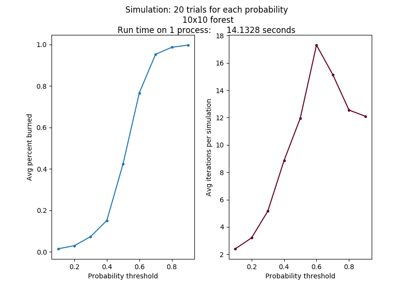
In this case, we ran 20 trials on a single Raspberry Pi 3B, with the probability threshold starting at 0.1 and incrementing by 0.1.

As the size of the grid changes and the probability points increase, this curve will look roughly the same, although it should get smoother as the number of trials increases and the increment value is smaller. But these more accurate simulations take a long time to run.

There are a couple of functions that a full simulation uses, and they are in the following code block for reference.

# # Functions used by both the sequential and MPI version of # the larger simulation with many trials. # # Libby Shoop Macalester College # import argparse # for command-line arguments def parseArguments(): """Handle command line arguments Run with -h to get details of each argument. Returns: A list containg each argument provided """ # process command line arguments # see https://docs.python.org/3.3/howto/argparse.html#id1 parser = argparse.ArgumentParser() parser.add_argument("numTreesPerRow", help="number of trees in row of square grid") parser.add_argument("probabilityIncrement", help="amount to increment the probability threshold of fire spreading for each set of probability trials") parser.add_argument("numberOfTrials", help="number of times to run the fire simulation with a new forest for each proability in set of probabilities") args = parser.parse_args() row_size = int(args.numTreesPerRow) prob_spread_increment = float(args.probabilityIncrement) num_trials = int(args.numberOfTrials) return [row_size, prob_spread_increment, num_trials] def burn_until_out(row_size, forest, prob_spread): """ one simulation of the buring forest Parameters: row_size (int): number of trees in each row and column forest (array): array representing the 2D forest prob_spread (float): probability threshold for determining whether burning tree will spread to neighboring tree """ percent_burned = 0.0 # for now start burning at midlle tree middle_tree_index = int(row_size/2) light_tree(row_size, forest, middle_tree_index, middle_tree_index) iter = 0 # how many iterations before the fire burns out while forest_is_burning(forest): # print("burning") # debug forest_burns(forest, row_size, prob_spread) iter += 1 percent_burned = get_percent_burned(forest, row_size) # print_forest(forest) #debug return int(iter), float(percent_burned)

Now here is the code for the single processor version of the simulation. It starts at a probability threshold of 0.1, then runs a set of trials using that threshold. Then it increases the threshold by a given increment amount and runs another set of trials. This is repeated until the threshold value is just below 1.0. For example, if the threshold increment is given as 0.1, the set of thresholds run will be:

0.1, 0.2, 0.3, 0.4, 0.5, 0.6, 0.7, 0.8, and 0.9

It takes three arguments in this order:

1. size of a row in a square forest of trees

2. amount to increment for each new probability threshold

3. number of trials to run at each threshold

# # Run multiple simulations of a fire burning at several probability thresholds. # # Ported to python from the original Shodor foundation example: # https://www.shodor.org/refdesk/Resources/Tutorials/BasicMPI/ # # Libby Shoop Macalester College # import argparse # for command-line arguments import math import time import numpy as np ############################# main() ########################## def main(): start = time.process_time() # start the timing row_size, prob_spread_increment, num_trials = parseArguments() # determine how many probabilities between .1 up to but not including 1.0 # will be tried, based on increment given on command line. tot_prob_trials = int(math.ceil((1.0 - 0.1)/prob_spread_increment)) # Note: num_trials simulations will be run, where an iteration # will be for tot_prob_trials. # print("total probability values : {}".format(tot_prob_trials)) #debug # set up result data arrays to hold: # sums of each value computed for each probability while iterating percent_burned_data = np.zeros( (tot_prob_trials, 2) ) iters_per_sim_data = np.zeros( (tot_prob_trials, 2) ) # The primary work: run the trials using each set of proabilities. # There will be num_trials x tot_prob_trials individual fire simulations # run, each with a new forest. for i in range(num_trials): idx = 0 # index into result data array for prob_spread in np.arange(0.1, 1.0, prob_spread_increment): forest = initialize_forest(row_size) iter, percent_burned = burn_until_out(row_size, forest, prob_spread) if i == 0: #put proability for x axis in result once percent_burned_data[(idx,0)] = prob_spread iters_per_sim_data[(idx,0)] = prob_spread #add data for this trial to running total for each trial percent_burned_data[(idx,1)] += percent_burned iters_per_sim_data[(idx,1)] += iter idx += 1 # find average percent burned and number of iterations # for each probability threashold for row in range(tot_prob_trials): percent_burned_data[(row,1)] = percent_burned_data[(row,1)]/num_trials iters_per_sim_data[(row,1)] = iters_per_sim_data[(row,1)]/num_trials finish = time.process_time() # end the timing total_time = finish - start print("Running time: {0:12.4f} seconds".format(total_time)) # Report data for the simulation results upper_title = "Simulation: {0} trials for each probability\n {1}x{1} forest\nRun time on 1 process: {2:12.4f} seconds" upper_title = upper_title.format(num_trials, row_size, total_time) print(upper_title) print("Average percent of trees burned at each probability:") print(percent_burned_data ) print("Average number of iterations per each probability:") print(iters_per_sim_data) ########## Run the main function main()

Warning

In this case, this program should run on only one process, so please do not change the -np mpirun flag.

Exercise

Run this with the default command line arguments given, which are 20x20 forest, increment probability threshold every 0.1, and run 10 trials. Note the time. Double the number of trials to 20 and note the time.

At this point if you increase the size of the forest or try to run more trials or more probabilities, the service that runs this code for you will time out.

Note

The message here is that running a simulation that would try to use a larger forest or get more accurate results (more trials, smaller probability threshold increments) is difficult to do with one processor.

The parallel MPI version

The desired outcome of the parallel version is to also produce data of average percent burns as a function of probability of spreading, as quickly and as accurately as possible. This should take into account that the probability of the fire spreading will affect not only how long it takes for the fire to burn out but also the number of iterations required to reach an accurate representation of the average.

If we put more processes to work on the problem, we should be able to complete a more accurate simulation in less time than the sequential version. Even the same problem as above can generate similar results running on 4 processes in almost 1/4 of the time.

The parallelization happens by splitting up the number of trials to be run among the processes. Each process completes the range of probabilities for its portion of the trials, sending the results back to the conductor process.

# Run multiple trial simulations of a fire burning at several # probability thresholds. # This version distributes the trials across multiple MPI processes. # # Ported to python from the original Shodor foundation example: # http://www.shodor.org/refdesk/Resources/Tutorials/BasicMPI/ # # Libby Shoop Macalester College # import math import time import numpy as np from mpi4py import MPI ############################# main() ########################## def main(): # MPI information comm = MPI.COMM_WORLD id = comm.Get_rank() #number of the process running the code numProcesses = comm.Get_size() #total number of processes running myHostName = MPI.Get_processor_name() #machine name running the code np.random.seed() # each process starts with seed from its /dev/urandom start = MPI.Wtime() # start the timing # conductor process will get the arguments # each process gets sent row_size, prob_spread_increment, and # its number of trials to perform (via a broadcast) if id == 0: # row_size, prob_spread_increment, tot_num_trials args = parseArguments() else: args = None # all processes participate in the broadcast sim_data = comm.bcast(args, root=0) # set the simulation values row_size = sim_data[0] prob_spread_increment =sim_data[1] tot_num_trials = sim_data[2] # determine number of trials that each process will do # by checking whether trials are divisible by number of processes # and if not spreading the work so that some do one extra trial remainder = tot_num_trials%numProcesses num_trials = int(tot_num_trials/numProcesses) if remainder !=0 and id >= numProcesses - remainder: num_trials += 1 # determine how many probabilities between .1 up to but not including 1.0 # will be tried, based on increment given on cammand line. tot_prob_trials = int(math.ceil((1.0 - 0.1)/prob_spread_increment)) # Note: tot_num_trials simulations will be run, where an iteration # will be for tot_prob_trials. # set up result data arrays to hold: # sums of each value computed for each probability while iterating percent_burned_data = np.zeros( (tot_prob_trials, 2) ) iters_per_sim_data = np.zeros( (tot_prob_trials, 2) ) # conductor holds arrays for receving data from workers if id == 0: recv_percent_burned_data = np.zeros( (tot_prob_trials, 2) ) recv_iters_per_sim_data = np.zeros( (tot_prob_trials, 2) ) # The primary work: run the trials using each set of proabilities. # There will be num_trials x tot_prob_trials individual fire simulations # run, each with a new forest. for i in range(num_trials): idx = 0 # index into result data array for prob_spread in np.arange(0.1, 1.0, prob_spread_increment): forest = initialize_forest(row_size) iter, percent_burned = burn_until_out(row_size, forest, prob_spread) if i == 0: #put proability for x axis in result once percent_burned_data[(idx,0)] = prob_spread iters_per_sim_data[(idx,0)] = prob_spread #add data for this trial to running total for each trial percent_burned_data[(idx,1)] += percent_burned iters_per_sim_data[(idx,1)] += iter idx += 1 # find average percent burned and number of iterations # for each probability threashold for row in range(tot_prob_trials): percent_burned_data[(row,1)] = percent_burned_data[(row,1)]/num_trials iters_per_sim_data[(row,1)] = iters_per_sim_data[(row,1)]/num_trials # each worker will send its computed data to the conductor, who receives # it in turn from each worker and updates its copy if id !=0: comm.Send(percent_burned_data, dest=0, tag=1) comm.Send(iters_per_sim_data, dest=0, tag=2) proc_time = MPI.Wtime() - start #uncomment the following to see how long each process takes #print("Process {0} ({1}) Running time: {2:12.4f} seconds".format(id, # myHostName, proc_time)) else: #conductor # get each worker's arrays and add the contents to its arrays for proc in range(1, numProcesses): comm.Recv(recv_percent_burned_data, source=proc, tag=1) comm.Recv(recv_iters_per_sim_data, source=proc, tag=2) for row in range(tot_prob_trials): percent_burned_data[(row,1)] += recv_percent_burned_data[(row,1)] iters_per_sim_data[(row,1)] += recv_iters_per_sim_data[(row,1)] # determine the averages for row in range(tot_prob_trials): percent_burned_data[(row,1)] = percent_burned_data[(row,1)]/numProcesses iters_per_sim_data[(row,1)] = iters_per_sim_data[(row,1)]/numProcesses # barrier here since conductor waited until all are finished sending if id == 0: #conductor will have overall time and can print the results finish = MPI.Wtime() # end the timing total_time = finish - start print("Total Running time: {0:12.4f} seconds".format(total_time)) # Report data for the simulation results upper_title = "Simulation: {0} trials for each probability\n {1}x{1} forest\nRun time on {2} processes: {3:12.4f} seconds" upper_title = upper_title.format(tot_num_trials, row_size, numProcesses, total_time) print("Average percent of trees burned at each probability:") print(percent_burned_data ) print("Average number of iterations per each probability:") print(iters_per_sim_data) ########## Run the main function main()

Exercises

1. Run the above with the defaults and compare the running time to the previous sequential example with the same settings. Is the time for 4 processes close to \(1/4\) the time using 1?

2. Try 40 trials, which should give us slightly more accurate averages.

3. To get more data and increase the trials, try using this for the command line arguments: [‘20’, ‘0.05’, ‘60’] and set the flags for mpirun to [-np 16’] to use 16 processes. Note how you can get more data using 16 processes in about the same time as the sequential version.

Try some other cases to observe how it scales

Ideally, as you double the number of workers on the same problem, the time should be cut in half. This is called strong scalability. But there is some overhead from the message passing, so we don’t often see perfect strong scalability.

Try running these tests and jot down your time values:

-np	tree row size	probability increment	number of trials	running time
2	20	0.1	40
4	20	0.1	40
8	20	0.1	40
16	20	0.1	40

What do you observe about the time as you double the number of processes?

When does the message passing cause the most overhead, which adds to the running time?

Try some other cases of your own design.

You have attempted of activities on this page