1.4 Real World Problem - Drug Design

Let’s look at a larger example. An important problem in the biological sciences is that of drug design. The goal is to find small molecules, called ligands, that are good candidates for developing into drug treatments.

The biology of drug design

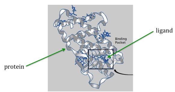
The proteins in our bodies have particular shapes that enable them to carry out the processes we need to live. Each protein consist of a long sequence of biological material, called amino acids, that naturally folds into a particular three-dimensional shape, according to the type of that protein. A disease may arise if something goes wrong with the shape of a type of protein. Ligands are shorter sequences of amino acids that fold into their own shapes. If a ligand can be discovered that binds (fits) into a target protein in order to change that protein’s shape in a beneficial way, then a drug supplying that type of ligand could treat a disease caused by that protein.

Here is an image illustrating the concept of a ligand (represented by small sticks in center) binding to the folded shape of a protein (represented by ribbon structure):

But how can the right ligands be found and formulated into drugs for treating diseases? Teams of laboratory scientists and medical professionals need years to develop and test new drugs. Fortunately software simulations can help identify favorable ligands for the laboratory scientists to work from, thus greatly reducing the time and costs for the design of drugs. The software assigns a matching score to each ligand that indicates how well they are likely to bind with the desired region of a (folded) target protein. The scientists can then start their laboratory work with the promising high-scoring ligands.

Problem Definition

Working with actual ligand and protein data is beyond the scope of this example, so we will represent the computation by a simpler string-based comparison.

Specifically, we simplify the computation as follows:

• Proteins and ligands will be represented as (randomly-generated) character strings.

• The docking-problem computation will be represented by comparing a ligand string L to a protein string P. The score for a pair [L, P] will be the maximum number of matching characters among all possibilities when L is compared to P, moving from left to right, allowing possible insertions and deletions. For example, if L is the string “cxtbcrv” and P is the string “lcacxtqvivg,” then the score is 4, arising from this comparison of L to a segment of P:

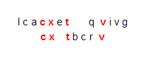
This is not the only comparison of that ligand to that protein that yields four matching characters. Another one is

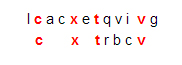
However, there is no comparison that matches five characters while moving from left to right, so the score is 4.

Implementations

The first example program below provides a sequential C++ implementation of our simplified drug design problem.

Note

The program optionally accepts up to three command-line arguments:

1. maximum length of the (randomly generated) ligand strings

2. number of ligands generated

3. protein string to which ligands will be compared

We will explore some example code that generates short strings, representing ligands, then assigns a score to each ligand according to how well it matches a longer string, representing a protein. In real drug design work, the scoring algorithms based on molecular biology are much more sophisticated than the example code’s simple matching algorithm. But for both the real software and our example code, the longer the ligand or the longer the protein, the longer it takes for the matching and score of the match to complete. Also, parallel computing can significantly speed up the computation time for our example code, as it does for real drug design software.

By default, we create a list of 100 possible ligands as random strings of length between 1 and 7. Below in the code box at the bottom of the code, the first command line argument represents the ligand length, and the second command line argument represents the number of ligands to try.

We have created a default fake protein in the example code. This can be changed on the command line by adding a third string, or you can update the code itself (see the tab for the MR class declaration).

In this implementation, the class MR encapsulates the map-reduce steps Generate_tasks(), Map(), and Reduce() as private methods (member functions of the class defined in the first tab for the MR class definition in the second tab), and a public method run() invokes these steps according to a map-reduce program strategy (in first tab below):

• A set of random ligands of varying lengths are put in a queue (Generate_tasks()).

• In a loop, the Map function computes a score for each ligand, creating a list of pairs containing the ligand and its score.

• The ligands are sorted according to their scores, highest first.

• The Reduce function keeps only the ligands with the highest score (multiple ones could have the highest score).

When you try running this, note that it takes several seconds to run, so be patient.

Warning

We advise that you keep the maximum length of 7 and 100 ligands as given, because you will likely exceed the time limit for this book’s code execution on the remote machine that this runs on.

// Main program int main(int argc, char **argv) { int max_ligand = DEFAULT_max_ligand; int nligands = DEFAULT_nligands; string protein = DEFAULT_protein; if (argc > 1) max_ligand = strtol(argv[1], NULL, 10); if (argc > 2) nligands = strtol(argv[2], NULL, 10); if (argc > 3) protein = argv[3]; // command-line args parsed double start, end, total_time; start = omp_get_wtime(); // timer begin MR map_reduce; // instance of our class // now run the simulation vector<Pair> results = map_reduce.run(max_ligand, nligands, protein); end = omp_get_wtime(); total_time = end - start; cout << "maximal score is " << results[0].key << ", achieved by ligands " << endl << results[0].val << endl; cout << "time: " << std::fixed << total_time << " seconds." << endl; return 0; } /* class MR methods */ ////////////////// run method where the work takes place const vector<Pair> &MR::run(int ml, int nl, const string& p) { max_ligand = ml; nligands = nl; protein = p; // put random ligands in a queue Generate_tasks(tasks); while (!tasks.empty()) { // score the next ligand Map(tasks.front(), pairs); tasks.pop(); } do_sort(pairs); // sort ligands by score // index of first unprocessed pair in pairs[] vector<Pair>::size_type next = 0; // find highest scoring ligand(s) while (next < pairs.size()) { string values; values = ""; int key = pairs[next].key; next = Reduce(key, pairs, next, values); Pair p(key, values); results.push_back(p); } return results; } //////////////////////// end run method void MR::Generate_tasks(queue<string> &q) { for (int i = 0; i < nligands; i++) { q.push(Help::get_ligand(max_ligand)); } } void MR::Map(const string &ligand, vector<Pair> &pairs) { Pair p(Help::score(ligand.c_str(), protein.c_str()), ligand); pairs.push_back(p); } bool compare(const Pair &p1, const Pair &p2) { return p1.key > p2.key; } void MR::do_sort(vector<Pair> &vec) { sort(vec.begin(), vec.end(), compare); } int MR::Reduce(int key, const vector<Pair> &pairs, vector<Pair>::size_type index, string &values) { while (index < pairs.size() && pairs[index].key == key) values += pairs[index++].val + " "; return index; } /* class Help methods */ // returns arbitrary string of lower-case letters // of length at most max_ligand string Help::get_ligand(int max_ligand) { int len = 1 + rand()%max_ligand; string ret(len, '?'); for (int i = 0; i < len; i++) ret[i] = 'a' + rand() % 26; return ret; } // recursive scoring function int Help::score(const char *str1, const char *str2) { if (*str1 == '\0' || *str2 == '\0') return 0; // both argument strings non-empty if (*str1 == *str2) return 1 + score(str1 + 1, str2 + 1); else // first characters do not match return max(score(str1, str2 + 1), score(str1 + 1, str2)); }

#include <iostream> #include <queue> #include <string> #include <vector> #include <algorithm> #include <cstdlib> #include <omp.h> #define DEFAULT_max_ligand 7 #define DEFAULT_nligands 100 #define DEFAULT_protein "the cat in the hat wore the hat to the cat hat party" using namespace std; // key-value pairs, used for both Map() out/Reduce() in and for Reduce() out struct Pair { int key; string val; Pair(int k, const string &v) {key = k; val = v;} }; // MR class provides map-reduce structural pattern class MR { private: int max_ligand; int nligands; string protein; queue<string> tasks; vector<Pair> pairs, results; void Generate_tasks(queue<string> &q); void Map(const string &str, vector<Pair> &pairs); void do_sort(vector<Pair> &vec); int Reduce(int key, const vector<Pair> &pairs, vector<Pair>::size_type index, string &values); public: MR() {} const vector<Pair> &run(int ml, int nl, const string& p); }; // Auxiliary routines class Help { public: static string get_ligand(int max_ligand); static int score(const char*, const char*); };

The Parallel OpenMP Version

To create an OpenMP parallel version the runs correctly, we have to make a couple of key changes:

1. The while loop that works through each generated ligand needs to be converted to a for loop so that the data decomposition pattern using a parallel for loop can be used to split the work onto threads.

2. The pairs of each ligand with their score must be held in a data structure that multiple threads can update concurrently by incorporating appropriate locking mechanisms. This is done by using a concurrent_vector container from the threaded building blocks (tbb) library.

The important portion of the code is line 66, where the pragma for OpenMP requests a parallel for loop.

Note

The third command line argument provided is the number of threads to use. Try running using 1, 2, 3, and 4 threads. Note the time for each thread by recording them. You will enter them later below.

////////////////////////////////// Main program int main(int argc, char **argv) { int max_ligand = DEFAULT_max_ligand; int nligands = DEFAULT_nligands; int nthreads = DEFAULT_nthreads; string protein = DEFAULT_protein; if (argc > 1) max_ligand = strtol(argv[1], NULL, 10); if (argc > 2) nligands = strtol(argv[2], NULL, 10); if (argc > 3) nthreads = strtol(argv[3], NULL, 10); if (argc > 4) protein = argv[4]; // command-line args parsed cout << "max_ligand=" << max_ligand << " nligands=" << nligands << " nthreads=" << nthreads << endl; #ifdef _OPENMP cout << "OMP defined" << endl; #else cout << "OMP not defined" << endl; #endif double start, end, total_time; start = omp_get_wtime(); // timer begin MR map_reduce; vector<Pair> results = map_reduce.run(max_ligand, nligands, nthreads, protein); end = omp_get_wtime(); total_time = end - start; cout << "maximal score is " << results[0].key << ", achieved by ligands " << endl << results[0].val << endl; cout << "time: " << std::fixed << total_time << " seconds." << endl; return 0; } ////////////////////////////////// end Main /* class MR methods */ /////////////////////// run method that forks threads ////// const vector<Pair> &MR::run(int ml, int nl, int nt, const string& p) { max_ligand = ml; nligands = nl; nthreads = nt; protein = p; Generate_tasks(tasks); // create ligands vector<string>::size_type t; // next task omp_set_num_threads(nthreads); // score each ligand ////////////////////////////// the OpenMP parallel for loop #pragma omp parallel for schedule(static) for ( t = 0; t < tasks.size(); t++) { Map(tasks[t], pairs); } do_sort(pairs); // index of first unprocessed pair in pairs[] tbb::concurrent_vector<Pair>::size_type next = 0; while (next < pairs.size()) { string values; values = ""; int key = pairs[next].key; next = Reduce(key, pairs, next, values); Pair p(key, values); results.push_back(p); } return results; } void MR::Generate_tasks(vector<string> &q) { for (int i = 0; i < nligands; i++) { q.push_back(Help::get_ligand(max_ligand)); } } void MR::Map(const string &ligand, tbb::concurrent_vector<Pair> &pairs) { Pair p(Help::score(ligand.c_str(), protein.c_str()), ligand); pairs.push_back(p); } bool compare(const Pair &p1, const Pair &p2) { return p1.key > p2.key; } void MR::do_sort(tbb::concurrent_vector<Pair> &vec) { tbb::parallel_sort(vec.begin(), vec.end(), compare); } int MR::Reduce(int key, const tbb::concurrent_vector<Pair> &pairs, vector<Pair>::size_type index, string &values) { while (index < pairs.size() && pairs[index].key == key) values += pairs[index++].val + " "; return index; } /* class Help methods */ // returns arbitrary string of lower-case // letters of length at most max_ligand string Help::get_ligand(int max_ligand) { int len = 1 + rand()%max_ligand; string ret(len, '?'); for (int i = 0; i < len; i++) ret[i] = 'a' + rand() % 26; return ret; } int Help::score(const char *str1, const char *str2) { if (*str1 == '\0' || *str2 == '\0') return 0; // both argument strings non-empty if (*str1 == *str2) return 1 + score(str1 + 1, str2 + 1); else // first characters do not match return max(score(str1, str2 + 1), score(str1 + 1, str2)); }

#include <iostream> #include <queue> #include <string> #include <vector> #include <algorithm> #include <cstdlib> #include <tbb/concurrent_vector.h> #include <tbb/parallel_sort.h> #include <omp.h> #define DEFAULT_max_ligand 7 #define DEFAULT_nligands 100 #define DEFAULT_nthreads 4 #define DEFAULT_protein "the cat in the hat wore the hat to the cat hat party" using namespace std; // key-value pairs, used for both Map() out/Reduce() in and for Reduce() out struct Pair { int key; string val; Pair(int k, const string &v) {key = k; val = v;} }; // MR class provides map-reduce structural pattern class MR { private: int max_ligand; int nligands; int nthreads; string protein; vector<string> tasks; tbb::concurrent_vector<Pair> pairs; vector<Pair> results; void Generate_tasks(vector<string> &q); void Map(const string &str, tbb::concurrent_vector<Pair> &pairs); void do_sort(tbb::concurrent_vector<Pair> &vec); int Reduce(int key, const tbb::concurrent_vector<Pair> &pairs, vector<Pair>::size_type index, string &values); public: MR() {} const vector<Pair> &run(int ml, int nl, int nt, const string& p); }; // Auxiliary routines class Help { public: static string get_ligand(int max_ligand); static int score(const char*, const char*); };

Exploring performance

On line 66 above, we used a clause for the parallel for loop pattern: schedule(static). This clause indicates that the work of processing each ligand in the for loop should be divided evenly among the threads.

After recording the times for this version for 1, 2, 3, and 4 threads, you can try changing the word ‘static’ inside the parentheses to dynamic, so it looks like this: schedule(dynamic). Then repeat this, collecting times for 1, 2, 3, and 4 threads.

Exercise 1:

You can write your results as a table that looks like this:

Time (s)	1 Thread	2 Threads	3 Threads	4 Threads
drugdesign-static
drugdesign-dynamic

Exercise 2:

Q-5: Time the static and dynamic versions of the drug design exemplar code on multiple threads (N=1..4). How does the runtime of the two versions compare?

• They take approximately the same time to run.
• No. Did you try and run the two examples?
• The static version performs better.
• Incorrect. Try re-running the code.
• The dynamic version perofrms better.
• Correct! The dynamic version of the code is significantly faster.

Exercise 3:

Recall that the equation for speedup is:

\[S_n = \frac{T_1}{T_n}\]

Where \(T_1\) is the time it takes to execute a program on one thread, \(T_n\) is the time it takes to execute that same program on n threads, and \(S_n\) is the associated speedup.

We will use Python to assist us with our speedup calculation. Fill in the code below to compute the speedup for each version on each set of threads:

#lists holding measured times (floating point) #TODO: Fill in arrays below (code will not compile otherwise!) # 1 2 3 4 dd_static = [ , , , ] dd_dynamic= [ , , , ] #compute speedup static_speedup = [round(dd_static[0]/dd_static[i],2) for i in range(1,4)] dynamic_speedup = [round(dd_dynamic[0]/dd_dynamic[i],2) for i in range(1,4)] print("static speedup:") print(static_speedup) print("dynamic speedup:") print(dynamic_speedup)

Summary

In many cases, static scheduling is sufficient. However, there is an implicit assumption with static scheduling that all components take about the same amount of time. However, if some components take longer than others, a load balancing issue can arise. In the case of the drug design example, different ligands take longer to compute than others. Therefore, a dynamic scheduling approach is better.

You have attempted of activities on this page