1.4 Real World Problem - Drug Design
Let’s look at a larger example. An important problem in the biological sciences is that of drug design. The goal is to find small molecules, called ligands, that are good candidates for developing into drug treatments.
The biology of drug design
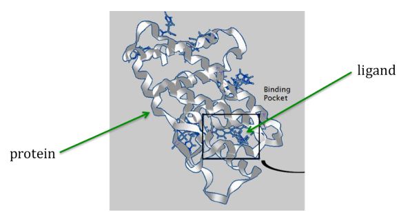
The proteins in our bodies have particular shapes that enable them to carry out the processes we need to live. Each protein consist of a long sequence of biological material, called amino acids, that naturally folds into a particular three-dimensional shape, according to the type of that protein. A disease may arise if something goes wrong with the shape of a type of protein. Ligands are shorter sequences of amino acids that fold into their own shapes. If a ligand can be discovered that binds (fits) into a target protein in order to change that protein’s shape in a beneficial way, then a drug supplying that type of ligand could treat a disease caused by that protein.
Here is an image illustrating the concept of a ligand (represented by small sticks in center) binding to the folded shape of a protein (represented by ribbon structure):
But how can the right ligands be found and formulated into drugs for treating diseases? Teams of laboratory scientists and medical professionals need years to develop and test new drugs. Fortunately software simulations can help identify favorable ligands for the laboratory scientists to work from, thus greatly reducing the time and costs for the design of drugs. The software assigns a matching score to each ligand that indicates how well they are likely to bind with the desired region of a (folded) target protein. The scientists can then start their laboratory work with the promising high-scoring ligands.
We will explore some example code that generates short strings, representing ligands, then assigns a score to each ligand according to how well it matches a longer string, representing a protein. In real drug design work, the scoring algorithms based on molecular biology are much more sophisticated than the example code’s simple matching algorithm (described here, in case you’re interested). But for both the real software and our example code, the longer the ligand or the longer the protein, the longer it takes for the matching and score of the match to complete. Also, parallel computing can significantly speed up the computation time for our example code, as it does for real drug design software.
We have created a default fake protein in the example code. This can be changed on the command line.
We create the list of possible ligands in 2 ways:
If the number of ligands is <= 18, the list of ligands comes from a fabricated list that is hard-coded in the code. We designed this as an example with a range of ligands whose length was from 2 through 6.
If the number of ligands is > 18, the ligands are generated randomly using a gamma distribution that looks like this:
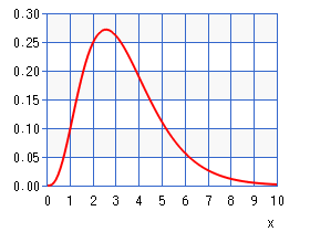
This means that we will have more ligands of length 2 or 3 and fewer of 4, 5, and 6, which are each declining in number. This has no relation to the real problem, but instead gives us some ligands that can be computed in a reasonable amount of time on a small cluster of single board computers. This way you can try some experiments and be able to see the advantage of one implementation over the other.
The image of the above Gamma distribution of lengths of ligands came from: this website, where we used a = 4.2 and b = 0.8.
The Serial Version
The serial version of the code is accessible at this link: dd_serial.cpp.
Compile the code locally on your machine using the following command:
g++ -o -o dd_serial dd_serial.cpp
To run the serial version of the program on your machine, run the following command:
time -p ./dd_serial
The Parallel Versions
There are two parallel versions of the code available:
A version that uses static scheduling and is implemented in OpenMP (
drugdesign_static)A version that uses dynamic scheduling and is implemented in OpenMP (
drugdesign_dynamic)
We will discuss static vs dynamic scheduling in greater detail later. For now, let’s compile the two version and run them:
g++ -o -o drugdesign-static drugdesign-static.cpp -fopenmp
g++ -o -o drugdesign-dynamic drugdesign-dynamic.cpp -fopenmp
You can measure the run-time of a particular iteration using time -p and specifying a number of threads. For example,
to run the static version of the drug design implementation on 2 threads use the command:
time -p ./drugdesign-static 2
Exercise 1:
Fill out the table by running the following series of tests:
Time (s) |
1 Thread |
2 Threads |
3 Threads |
4 Threads |
|---|---|---|---|---|
drugdesign-static |
||||
drugdesign-dynamic |
Exercise 2:
- They take approximately the same time to run.
- No. Did you try and run the two examples?
- The static version performs better.
- Incorrect. Try re-running the code.
- The dynamic version perofrms better.
- Correct! The dynamic version of the code is significantly faster.
Q-1: Time the static and dynamic versions of the drug design exemplar code on multiple threads (N=1..4). How does the runtime of the two versions compare?
Exercise 3:
Recall that the equation for speedup is:
Where \(T_1\) is the time it takes to execute a program on one thread, \(T_n\) is the time it takes to execute that same program on n threads, and \(S_n\) is the associated speedup.
We will use Python to assist us with our speedup calculation. Fill in the code below to compute the speedup for each version on each set of threads:
Summary
In many cases, static scheduling is sufficient. However, there is an implicit assumption with static scheduling that all components take about the same amount of time. However, if some components take longer than others, a load balancing issue can arise. In the case of the drug design example, different ligands take longer to compute than others. Therefore, a dynamic scheduling approach is better.